7 minutes
A summary of my Master’s Thesis - as simple as it gets!

After spending four months working into a specific topic for a thesis, including literature review, recent papers and experimental evaluation, one tends to undervalue the depth of gained expertise in that specific area. Trying to formulate the thesis into simple words to explain to friends and family then presents a surprisingly difficult challenge. With a little more thought, I am therefore summarizing my Master’s thesis “Bayesian vs. PAC-Bayesian Ensembles” for everyone, regardless their background, in an article that (hopefully) only requires a couple of minutes, rather than hours, to read.
Broadly speaking, my thesis touched upon the area of Deep Learning, which is a subfield of Machine Learning. Machine Learning, at a high level, tries to teach a computer model a desired behavior by using data and statistical learning algorithms rather than explicitly programming the behavior. As a popular example, the desired behavior could be classification of a given image into different classes (e.g. animals). Instead of explicitly programming how to recognize a dog (which would be rather cumbersome and error-prone), the computer is fed thousands of pictures of dogs and learns how to recognize them. Deep Learning uses deep neural networks as models, which have proven efficient and highly accurate in a variety of applications, especially with images. The output of a model, when given a new image, is then the predicted class (often expressed with a probability, e.g. 80% “dog” and 20% “not dog”). Deep neural networks are, roughly speaking, built from neurons that are connected to each other with varying strengths. The strength of a connection is expressed as a “weight”, which has a value that is changed during training to optimize the model’s performance. After training, the weights are fixed and the model can be used to classify new and unknown inputs.
Taking the outputs of a model as single truth can be dangerous, especially if the decision is safety-critical or highly risky (e.g. medical diagnosis or self-driving). One never knows if/when a model might fail to perform its task and misclassify an input. One idea to avoid this issue: Just take multiple models’ outputs (those can be trained on the same data or on different data of the same type of problem) and combine their predictions, for example by a majority vote. This has been shown to improve performance and is known as an “ensemble”. A convenient side-effect of an ensemble is a better estimation of uncertainty: If most ensemble members disagree, one should be careful when using the prediction. In contrast, when all models conform, one can be quite certain that the output is correct.
Now, there is another approach called “Bayesian ensemble” that intends to improve uncertainty estimation in Machine Learning. It is based on Bayes’ law, which I will try to introduce as briefly as possible, with an example inspired by Daniel Kahneman’s book “Thinking, fast and slow”: Imagine that you read a statement about a man’s character, who you randomly pick from the population: “neat, tidy, introverted, order-loving”. Given the possible job options “farmer” and “librarian”, which one would you choose? If you think like me (and most others, I would argue), you’ll choose librarian, as those traits are typically more likely to find in a librarian than in a farmer. However, Bayes’ law teaches us that this disregards the fact that there are far more farmers than librarians in the general population. This knowledge is given before picking the person and is therefore called prior knowledge. Combined with the observation (here the person’s character statement), we obtain so-called posterior knowledge. This could then indicate that the probability that the man is a farmer is higher, because the number of farmers that fit the description is higher than the number of librarians, just because there are more farmers to begin with.
Returning to the thesis, Bayes’ law is applied to a deep neural network by expressing the weights as posterior knowledge, meaning that we do not adjust and fix them after the training, but express them as a probability distribution. More specifically, we express prior knowledge about the weights as a range of values where we would expect them to be after training. The observation here is the training data, and the posterior expresses for each weight, where its true value most likely is. Here, an ensemble can be formed by using this posterior from each weight to sample neural networks with different configurations (i.e., fixed settings of weights), and again combining their predictions as with the other ensemble before.
If you haven’t fully understood Bayesian ensembles described above, this is completely fine. The take-away can be summarized as: We don’t want to have one network with fixed weights after training, so we place a probability distribution over all possible networks and combine the predictions of a limited number of them to estimate how certain we can be about the prediction.
Now: The core of the thesis was a comparison between the mentioned ensemble approaches (Bayesian ensembles and “traditional” ensembles) theoretically and with experiments and evaluate their suitability when we care about prediction performance (i.e. disregarding the uncertainty estimation part). The term “PAC-Bayesian” that is found in the title, even though it sounds similar to “Bayesian”, describes how the influence of different members in a normal ensemble can be further improved by adjusting their contributions to the majority vote. I’ll leave out the details, but essentially, PAC-Bayesian ensembles are normal ensembles with a difference in weighting of the members.
I will now come to the results of the thesis. The theoretical comparison highlighted that normal ensembles are supposedly better suited to improve performance, as they combine multiple network’s outputs and theoretically cancel out each other’s mispredictions, such that the majority is more often right than any single member. Bayesian ensembles on the other hand, with more data, will not utilize this strength, as the posterior can be shown to collapse into a single model, i.e. the probability distribution for each weight approaches a probability that is 1 for only one value and 0 for all others. When sampling this distribution repeatedly to create an ensemble, all members will be the same, also meaning that the ensemble is only as good as each of its members. Highlighting that difference included the application of a well-known and already proven theorem (the Bernstein-von Mises theorem), and only served as a theoretical foundation for the experiments that followed after.
So, the experiments and their results might be the most tangible in this post. Overall, we could show that traditional ensembles (with equal and PAC-Bayesian optimized member influence) can beat and even outperform Bayesian ensembles, while they have a much simpler ensemble architecture (i.e. just train multiple networks and combine them), which can even be parallelized. A disadvantage of the PAC-Bayesian approach was the need for more training data, as a separate dataset needs to be taken to adjust the member influence in the ensemble. However, we also showed how this disadvantage can be overcome in cases where a separate dataset is used to select the best model from a model training run (a so-called validation set): We include multiple versions from the training history of each model into the ensemble (there can be good and bad ones), save the validation data, and use it instead to optimize the member influence, which we showed “filtered out” the bad models anyway
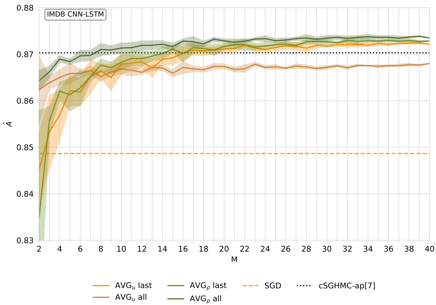
An exemplary figure of one of the experiments is shown below. “cSGHMC-ap[7]” is just the abbreviation for this specific Bayesian ensembling method including 7 models. All other lines are variations of traditional ensembles with equal and optimized member influence. It is observable that 3/4 configurations match and eventually outperform the reference in terms of accuracy on this classification task after exceeding a certain ensemble size M.
Well, that was more or less it. Of course, I left out some details, but I hope that the general idea and motivation of the thesis has become clear. It is often manageable to explain the background and general topic of a thesis, but including results and newly added insights to the academic community requires more depth, which is hopefully still making sense and built upon the brief foundations I gave. In case not - I guess you will just have to ask! And to everyone making it that far: Thank you for showing interest in the stuff I did at university!